This post provides a brief review of a paper by Dutta and Chaudhuri. The paper proposes an algorithm for RGB image edge detection. The proposed algorithm uses functions also in use in state-of-the-art methods today. For demonstration, I code the algorithm from scratch and compare it with state-of-the-art methods.
Overview
Edge detection is a fundamental tool in computer vision. It reduces data, while preserving useful structural information about object boundaries. A greyscale image contains about 90% of the edge information of its RGB correspondence; the remaining 10% can be crucial. The paper proposes a method which consists of smoothing, directional color difference calculation, thresholding and thinning (Soumya Dutta, 2009).
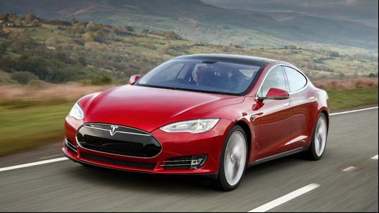
To test the algorithm, I use an image of a beautiful red Tesla Model S (Figure $1$). I will go through the algorithm step by step.

Adaptive median filter
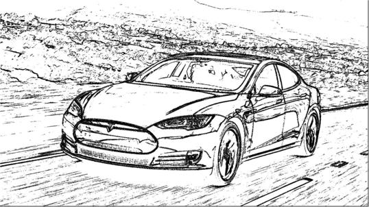
The Median filter is widely used in computer vision applications. It has great noise reduction capabilities for impulse noise, also called the “salt and pepper” noise. It works by moving a window over an image, where each pixel is located at the center of the window once (assume appropriate padding). Output at each pixel is the median of values within the window. As one might think, each color channel is operated separately. A problem with the median filter is that it does a poor job at preserving detail of an image while smoothing the non-impulse noise. The paper proposes an adaptive median filter to alleviate this problem. Intuitively, it additionally verifies which pixels are noise and which are not. An interested reader can find pseudocode of the adaptive median filter algorithm in the paper (Soumya Dutta, 2009).
Effect of the adaptive median filter is shown in (Figure $2$). Difference between the original and filtered image is subtle. The latter appears little smoother.
Directional masks
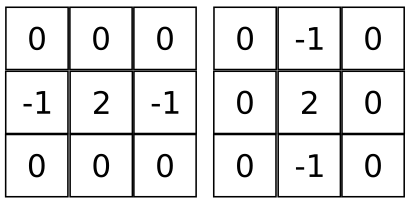
Directional color difference calculation (image gradients) is a critical part of the proposed algorithm. It locates areas where abrupt changes of RGB values occur; this is where the edges are! Roughly speaking, edges exist in four directions; horizontal, vertical, ascending and descending diagonal. The four directions are represented by masks or filters. The masks proposed by the paper are illustrated in (Figure $3$) (Soumya Dutta, 2009).

Before applying the masks, pixels are transformed to single valued attributes. The transformation is achieved by weighted addition of RGB components, as
$Pixel(i,j) = 2 * red(i,j) + 3 * green(i,j) + 4 * blue(i,j)$.
The masks are applied as a convolution with the image. The operator flips the mask horizontally and vertically (transpose). Then the flipped mask moves over the image, taking the Hadamard product (elementwise multiplication) between the current window and the mask at each location. The elements of a resulting matrix are summed up. At each location there are four results as there are four masks which are applied separately. The paper suggests to choose the largest resulting value as output. The output values build the gradient image.

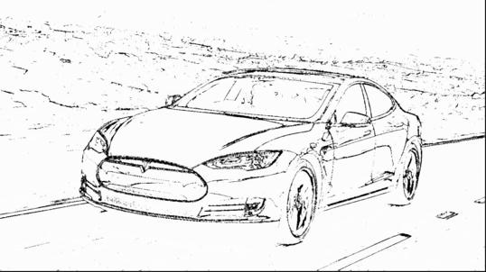
(Figure $4$) shows the effect of directional color difference calculation on the previously filtered image. At this point, the image background resembles static of an old television. Outlines of the Tesla and the road are there though!
Thresholding
Thresholding operation is straightforward. It is responsible for producing the visual edge map from the gradient image. In the algorithm, we choose a threshold, and turn every pixel smaller than the threshold white and every pixel larger than equal to the threshold black. That’s really all it is. The paper suggests a threshold of $1.2t$, where $t$ is an average value of maximum color difference. In other words, $t$ is equal to the average value of the gradient image.
(Figure $5$) shows the effect of thresholding on the gradient image. The result is already a quite decent edge map. The edges are still somewhat thick though, and there is some noise as well.
Thinning
Thinning alleviates the problem seen in (Figure $5$) to some degree. Thinning thins the thickest edges and the thinnest edges and dots will disappear. This means it tries to keep the most important edges and get rid of the most spurious edges.
Two masks are used in thinning (Figure $6$). One mask works in the horizontal direction and another in the vertical direction. The masks are applied as a convolution with the image.
(Figure $7$) is the final edge map produced by the proposed algorithm. It removes many unwanted dots and spurious edges from the previous step.
Comparison and conclusion
OpenCV Canny is a popular implementation of Canny edge detection algorithm. The algorithm is one of state-of-the-art edge detectors available today. The paper uses Canny as well to compare the methods.
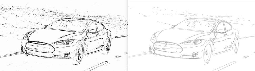
(Figure $8$) summarizes the results. To conclude, the proposed algorithm is able to produce edge maps which are comparable with the state-of-the-art method. OpenCV Canny still does little better job at getting rid of unwanted dots. It also presents the edges finer. I believe these minor differences partly stem from the thresholding algorithm in OpenCV Canny. It uses Hysteresis Thresholding, which outperforms the one proposed in the paper.