Bias in image datasets

Bias in image data, as described by Selvaraju et al., refers to a class exclusively containing visual information irrelevant to the class prediction. A ConvNet model trained on a vehicle dataset can learn the characteristics of different vehicles if it is focusing on vehicles. Now imagine images of vans exclusively containing people. The model likely learns to associate some parts of the people with vans (Figure $1$) and thus confidently classifies people as vans.

Figure 1. (Left) how my ConvNet tries to classify a van after training 50 epochs on a custom dataset of 4000 images. The dataset contains four classes; a van, car, semi and pickup truck. The data is divided equally between the classes, but the images of vans also contain people more often than other classes. Thus the ConvNet learns to associate the waist of the guy with vans. After mitigating this problem by adding more images to the dataset and removing the particular bias, the model (right) learns vans' characteristics.

Bias in datasets cause problems. Bias tends to be more common in smaller scale datasets because generally there’s less variety in data. However, larger datasets can suffer from bias as well. According to my own experience, the problem is often subtle and difficult to spot with human eye without any insights into the model (what the model sees). If the model struggles to generalize well (gap between training accuracy and test accuracy, validation accuracy might still be good), bias in the dataset might explain it. In the biased case the data generating distributions for training and testing are different. Quite expectedly the model performs poorly during the testing phase as it has not learned the same or even closely similar data distribution. Fortunately some bias in datasets can be detected by observing gradient information flowing into the last convolutional layer of the model. Selvaraju et al. takes advantage of this technique in their Grad-CAM algorithm.

Grad-CAM algorithm

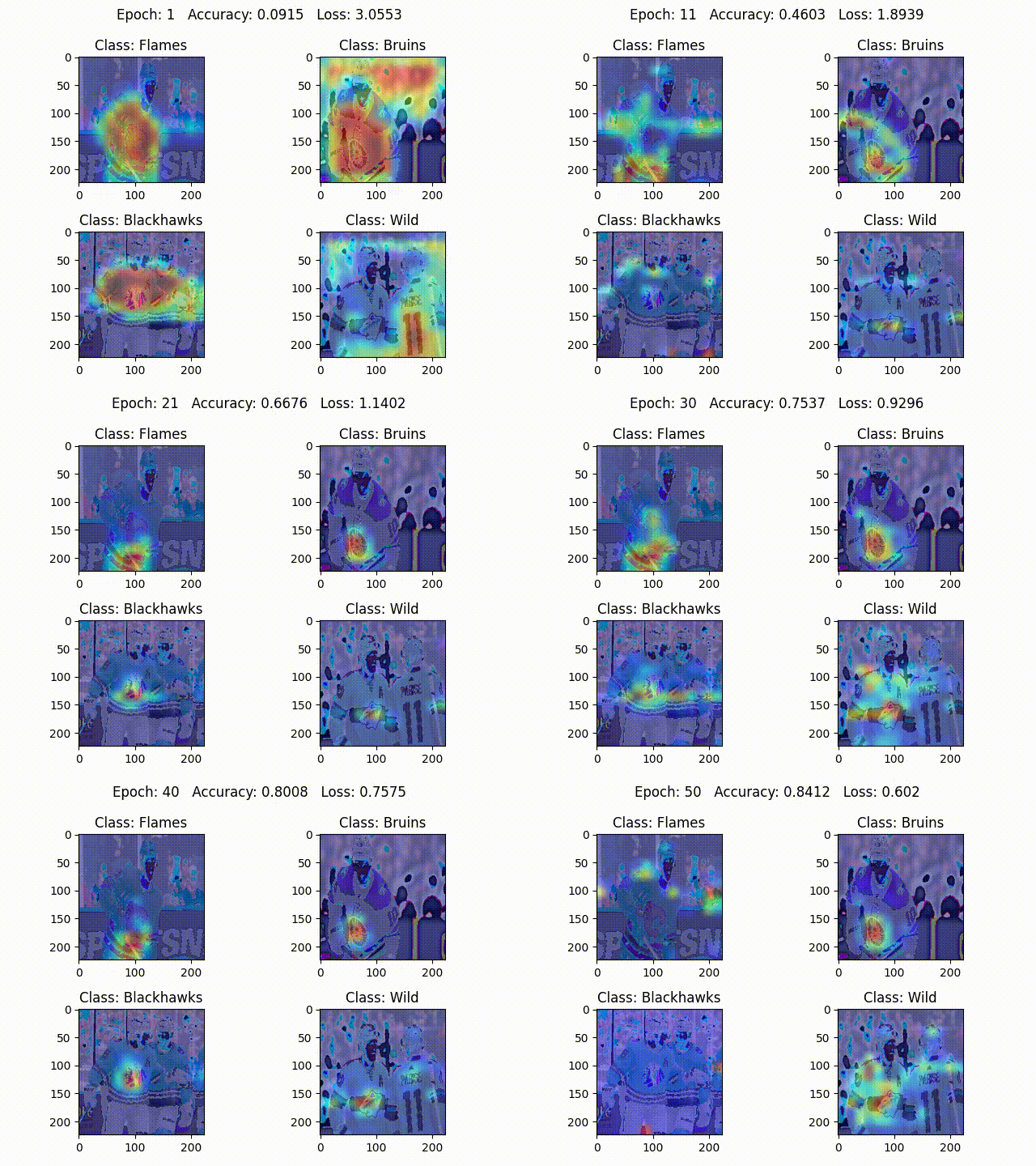
It is known that deeper representations in a ConvNet capture higher-level information from images such as object parts. Grad-CAM utilizes information from the gradients flowing into the last convolutional layer, where the deepest representations reside. The algorithm could be modified to use information from earlier convolutional layers as well, but the last convolutional layer decision making is visually most similar to how humans recognize objects. Intuitively, Grad-CAM looks at an image and tells how important each pixel in the image is for classifying it as a particular class (In Figure $2$, ConvNet is mainly focusing on logos and stripes to classify between the teams).

Figure 2. Recording what your ConvNet sees during training through Grad-CAM can help diagnose problems early. Red regions contain pixels that are important in decision making for a particular class in the example images, while blue regions do not contribute to decision making for the particular class.

The math behind the algorithm is quite elegant. Grad-CAM is defined as

where

What’s happening in (1) inside the Rectified Linear Unit (ReLU), we perform a linear combination of activation feature maps $\color{Blue}{A^{k}}$, where each activation feature map is weighed by an importance value $\color{DarkRed}{a_{k}^{c}}$. This importance value tells how important a feature map $\color{DarkRed}{k}$ is for a target class $\color{DarkRed}{c}$ when making a prediction. The linear combination of activation feature maps is likely to contain both negative and positive values. We are only interested in the features which have a positive influence on the class of interest $\color{Red}{y^{c}}$. Consequently, we apply ReLU to the result to turn negative values into zeroes. This results in a coarse heatmap which is the same size as the activation feature maps in the last convolutional layer.

So far very straightforward. Now what are the importance values $\color{DarkRed}{a_{k}^{c}}$? In $\color{Red}{\frac{\delta y^{c}}{\delta A_{ij}^{k}}}$ we use calculus to calculate the gradient of the score $\color{Red}{y^{c}}$ with respect to feature map activations $\color{red}{A_{ij}^{k}}$. In other words, we are checking how much a feature map contributed to the prediction of the class of interest. These values are global-average pooled in $\color{magenta}{\frac{1}{Z} \sum_{i} \sum_{j}}$ to obtain the final importance value, which tells us how we should weigh the specific activation feature map (Ramprasaath Selvaraju, 2019).

Reducing bias

As we have diagnosed the bias in our dataset, the next step is to do something about it. We want to get rid of the bias as much as we can. To counteract the bias we add images to the dataset which ensure that the other classes have the same “biased elements”. Assume we have an image dataset of some car models and one of the classes contain clouds in the background while others don’t, it is quite likely that the model will learn to associate the clouds with the specific car model. Now if the images of cars of the other classes also contain clouds in the background, there is less bias in the dataset and the model shouldn’t associate clouds with the same car model. Generally, collecting a bigger balanced dataset reduces bias. However, a big dataset does not guarantee an unbiased model. Collecting data and building a dataset is an art in itself.

Conclusion

This essay briefly talks about bias in image datasets and summarizes Grad-CAM algorithm. Bias in this context is a problem more common in smaller datasets. It affects ConvNet’s generalization ability and is often hard to detect without understanding what the model sees because of its subtle nature. Grad-CAM algorithm creates heatmaps of the same size as the original images, which visually show the regions that contributed to the prediction most. After diagnosing the bias, what follows is a straightforward method to reduce it. If you are not familiar with bias in image data already, this essay helps you get started. Beyond reading I encourage you to code Grad-CAM from scratch to get a deeper understanding why it works.